Module H · Backtesting, ML & Portfolio Construction - Chapter 70

Machine Learning in Quant: Promise and Peril

Where machine learning genuinely helps a quant, where it quietly leaks the future, and how to use it without fooling yourself.

NSE

What you'll learn

·Where ML helps vs hurts
·Train/test on time series
·Feature and label leakage
·Tree models vs linear
·Feature importance
·Avoiding overfit ML

Machine learning is the most hyped and most misunderstood tool in modern trading. The pitch is seductive: feed a powerful model enough data and it will discover patterns no human could see. The reality, in markets, is harsher - ML is brilliant at finding patterns that aren't there, fitting noise so convincingly that it fools its own creator. Used carelessly (which is how it's usually used), it's a faster, more sophisticated way to overfit. Used with discipline, it has a real but narrow place. This chapter is the honest overview: where ML genuinely earns its keep, where it quietly destroys capital, and the handful of habits that separate the two.

The honest experiment

Let's just try it. We'll build sensible features from past returns, momentum and volatility, and train a random forest to predict whether Nifty rises tomorrow - with a strict time-ordered split, no peeking:

EX 1An ML direction predictorINDEXch70/01_ml_classifier.py

# Can ML predict tomorrow's direction? Train honestly on time-ordered data and see.
import os
from datetime import datetime

import pandas as pd
from openalgo import api
from sklearn.ensemble import RandomForestClassifier

client = api(
    api_key=os.getenv("OPENALGO_API_KEY", "your_api_key_here"),
    host=os.getenv("OPENALGO_HOST", "http://127.0.0.1:5000"),
)

end = datetime.now().strftime("%Y-%m-%d")
c = client.history(symbol="NIFTY", exchange="NSE_INDEX", interval="D",
                   start_date="2019-01-01", end_date=end)["close"]
r = c.pct_change()

df = pd.DataFrame(index=c.index)
for lag in [1, 2, 3, 5]:
    df[f"ret{lag}"] = r.shift(lag)              # only PAST returns as features
df["mom10"] = c.pct_change(10).shift(1)
df["vol10"] = r.rolling(10).std().shift(1)
df["target"] = (r.shift(-1) > 0).astype(int)    # did tomorrow go up?
df = df.dropna()

X, y = df.drop(columns="target"), df["target"]
split = int(len(df) * 0.7)                       # time-ordered split - NEVER shuffle a time series
model = RandomForestClassifier(n_estimators=200, max_depth=5, random_state=0)
model.fit(X[:split], y[:split])

train_acc = model.score(X[:split], y[:split]) * 100
test_acc = model.score(X[split:], y[split:]) * 100
baseline = max(y[split:].mean(), 1 - y[split:].mean()) * 100

print(f"Train accuracy             : {train_acc:.1f}%")
print(f"Test accuracy (out-of-sample): {test_acc:.1f}%")
print(f"Baseline (always guess majority): {baseline:.1f}%")
print("\nHigh train, ~coin-flip test = the model memorised noise. Direction resists ML prediction.")

Live output

Train accuracy             : 69.1%
Test accuracy (out-of-sample): 50.1%
Baseline (always guess majority): 51.2%

High train, ~coin-flip test = the model memorised noise. Direction resists ML prediction.

Read those three numbers and feel the disappointment that every quant must internalise. The model hit 69% on the training data - it looks like it learned something. But on the out-of-sample test it scored 50% - a coin flip - and actually below the 51% you'd get by blindly guessing the majority class. The 69% was pure illusion: the model memorised the noise of the training period, which tells you nothing about tomorrow. A powerful algorithm, sensible features, clean code - and zero predictive edge on direction.

The overfit gap

The danger gets worse the more powerful the model. Let the trees grow deeper and watch the gap between training and reality explode:

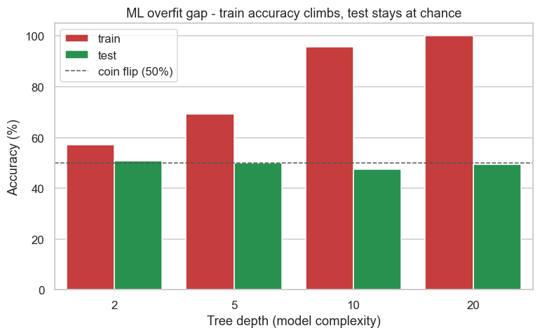
At the deepest setting the model scores a perfect 100% on training and 49% on test. That's the signature of overfitting in one chart: more complexity makes training accuracy soar and out-of-sample accuracy stay pinned at chance. In a low-signal domain like markets, model power is a liability - it just lets the model memorise more noise. This single picture should make you suspicious of any complex ML strategy that doesn't show its out-of-sample numbers.

Where ML helps and where it hurts

So is ML useless for quants? No - but you have to point it at the right problems:

ML's narrow, real place in a quant's toolkit

ML shines at combining many weak signals into one, capturing nonlinear interactions a linear model misses, forecasting volatility (which, unlike direction, has real structure - Chapter 42), and digesting alternative data like news text. It fails - dangerously - at predicting raw direction in low-signal data, exactly where beginners point it first.

Trees versus linear models

Why does a random forest keep showing up in quant ML when a humble linear regression is so much easier to reason about? Because the two make opposite bets. A linear model assumes each feature pushes the prediction in a straight line and the effects simply add up. It has few parameters, it is transparent (one coefficient per feature), and it is hard to overfit - which in a low-signal world is a genuine virtue. Its weakness is that it cannot see interactions: it cannot learn that momentum matters only when volatility is low, because that is a product of two features, not a sum.

A tree-based model - a single decision tree, or an ensemble of them like a random forest or gradient-boosted trees - does the opposite. It carves the feature space into rectangular regions with a cascade of yes/no splits, so it captures nonlinearities and interactions for free, needs no feature scaling, and shrugs off outliers and monotone transforms. That same flexibility is exactly why it overfits so eagerly on noisy financial data, as the last example showed. The practical rule on most tabular market problems: start with a regularised linear model as the honest baseline, then reach for gradient-boosted trees only when you can show, out-of-sample, that the nonlinearity actually pays. If the tree cannot beat the line on held-out data, the nonlinearity was noise.

Tip

Always quote a simple baseline next to your fancy model - a linear model, or even "predict the majority class". An ML result is only meaningful as the gap over a baseline. A 53% classifier sounds clever until you learn the majority class alone scores 53%.

Reading feature importance, and its traps

One reason trees are popular is that they hand you a feature importance ranking: a score for how much each input contributed to the model's splits. It feels like insight - a tidy list of which signals "matter". Treat that feeling with suspicion. The default scikit-learn importance (mean decrease in impurity, MDI) is computed on the training data, so it rewards whatever helped the model memorise noise, and it is biased toward high-cardinality, continuous features that simply offer more places to split. A feature can top the importance chart and carry zero out-of-sample edge.

The more trustworthy measure is permutation importance: shuffle one feature's column on the held-out set and measure how much the test score drops. If scrambling a feature does not hurt out-of-sample accuracy, that feature was not really pulling its weight, however high its MDI. Two cautions even then. Importance is not causation - a feature can rank high only because it proxies for something else. And when two features are strongly correlated, the importance gets split or double-counted between them, so a genuinely useful signal can look weak just because a near-twin is standing next to it.

Heads up

A feature importance chart describes your model, not the market - it tells you what the model leaned on, including the noise it leaned on. Never promote a feature to "this drives returns" on the strength of training-set importance alone; confirm it with permutation importance on data the model never saw.

Train and test on time, never shuffle

Everything above rests on one discipline that ML beginners break first: never shuffle a financial time series. Standard ML cross-validation randomly shuffles rows into folds. On market data that is catastrophic, because it lets the model train on days that come after the days it is tested on - a built-in leak from the future. Always split by time: train on the past, test on a later, untouched stretch, exactly as the examples above did. The rigorous versions are walk-forward validation and purged cross-validation (Chapter 69), which step the test window forward through time and delete the overlapping samples that would otherwise straddle the train-test boundary. Time order is sacred.

That same future-peeking is the deeper, more treacherous bug in financial ML: leakage - information that was not actually available at decision time seeping into training. It hides in a feature computed with data from after the prediction point, in labels that overlap across rows, or in scaling and feature-selection done over the whole dataset including the test rows. Leakage is to ML what look-ahead bias (Chapter 68) is to backtesting: the same disease, with far more places to hide. It is so central, and so entangled with how you build features and define labels, that the entire next chapter is devoted to it - constructing honest, point-in-time, stationary features, labelling trades the way they actually play out (the triple-barrier method), and the most successful pattern of all, meta-labeling, where a simple economic rule picks the direction and ML is asked only to filter and size it. For now, hold one rule above all the model-tuning: if your out-of-sample numbers look wonderful, suspect a leak before you believe the edge.

Key idea

In markets, model power is usually a liability - it overfits noise (train 100%, test 49%). ML's real value is narrow: combining weak signals, modelling volatility, processing alt-data, and filtering and sizing an economically grounded signal rather than calling raw direction. Always validate time-ordered, quote a simple baseline, read feature importance via permutation on held-out data, and hunt relentlessly for leakage.

Try it yourself

Shuffle the train/test split (the wrong way) and watch the test accuracy jump - proof of why time order matters.
Point the model at volatility instead of direction (predict whether tomorrow's |return| is large). Does ML do better on the predictable target?
Replace the random forest with a plain logistic regression on the same features. Does the simpler, linear model actually lose much - or anything - out-of-sample?

Recap

ML is brilliant at fitting noise: a random forest hit 69% (then 100%) in training but 50% / 49% out-of-sample - no edge on direction.
More model complexity widens the overfit gap in low-signal markets - power is a liability, not an asset.
ML helps with combining weak signals, nonlinear patterns, volatility forecasting and alt-data; it hurts at predicting raw direction.
Trees vs linear: linear models are transparent and hard to overfit but miss interactions; trees capture nonlinearity but overfit eagerly - earn the complexity out-of-sample.
Feature importance describes the model, not the market - confirm it with permutation importance on held-out data, never training-set MDI.
Split by time, never shuffle; leakage is the silent killer, and features, labels and leakage audits are the whole of the next chapter.

Used well, ML in markets is won or lost long before the model is fitted - in how you build the features and define the labels it learns from. That unglamorous, decisive craft - point-in-time features, stationary transforms, triple-barrier labels and the leakage audits that keep them honest - is exactly where we go next.