Backtesting Without Fooling Yourself

The backtest is the most powerful tool a quant owns, and the easiest way ever invented to lie to yourself. A few subtle, almost invisible mistakes can turn a worthless or even losing strategy into an equity curve so beautiful you will wire real money against it. This module is about earning the right to trust a backtest. This opening chapter lays out what a backtest actually is, the places it deceives you, and what a trustworthy one looks like. The two chapters that follow drill into the specific failure modes: the biases hiding in the data itself (Chapter 68) and the biases hiding in how you validate (Chapter 69).

The anatomy of a backtest

Strip away the framework and every backtest is the same short pipeline. Historical data feeds a signal - a rule that says long, short or flat at each moment. The signal is turned into fills at some assumed price. Those fills are charged costs. Fills and costs roll up into positions and P&L. And the P&L is compressed into a handful of metrics - Sharpe, drawdown, hit rate - that you judge the whole thing by.

Each link is honest only if the one before it was. A leaked price in stage one, a free fill in stage three, a forgotten cost in stage four - any single slip and the metrics in stage six describe a market that never existed. Most of this module is really about defending each of these stages in turn.

Realistic fills and costs

The most common way a beginner's backtest flatters itself is by assuming perfect, free execution. Two assumptions usually hide here. First, the fill price. You cannot buy at the exact close that generated your signal - by the time the bar closes and the rule fires, that price is gone. A defensible default is to act at the next bar's open, and to assume you pay at least half the spread to cross. Limit-order strategies have the opposite problem: you must model the fills you did not get, not just the ones you did.

Second, costs, and India's stack is heavy. Securities transaction tax, stamp duty, exchange and SEBI fees, GST and brokerage make up the all-in charge model of Chapter 8, and on top of that you pay the bid-ask spread and your own market impact to get filled at all (the liquidity and impact-cost work of Chapters 25 and 26). High-turnover strategies are especially brutal here: a rule that looks glorious gross can be a steady loser once every round trip is taxed and slipped. You must backtest net, always.

How a backtest fools you

The deepest deceptions are not in the costs but in timing and selection. The classic is look-ahead bias: letting the backtest use information it could not have had at the moment it traded. It is usually a one-line slip - forgetting to lag the signal, so the strategy decides today's trade using today's closing price, which it could not possibly know until the day was already over. Watch what that single error does to a plain moving-average rule on NIFTY:

# Look-ahead bias: forgetting to lag the signal by one bar fakes a brilliant edge.
import os
from datetime import datetime

import numpy as np
from openalgo import api

client = api(
    api_key=os.getenv("OPENALGO_API_KEY", "your_api_key_here"),
    host=os.getenv("OPENALGO_HOST", "http://127.0.0.1:5000"),
)

end = datetime.now().strftime("%Y-%m-%d")
c = client.history(symbol="NIFTY", exchange="NSE_INDEX", interval="D",
                   start_date="2021-01-01", end_date=end)["close"]
r = c.pct_change()

sma = c.rolling(20).mean()
signal = np.sign(c - sma)        # +1 above the average, -1 below (uses today's close)


def sharpe(x):
    x = x.dropna()
    return x.mean() / x.std() * np.sqrt(252)


cheat = sharpe(signal * r)          # BUG: trade today's return with today's signal
honest = sharpe(signal.shift(1) * r)  # correct: decide on yesterday's close, trade today

print(f"With look-ahead (signal * today's return) : Sharpe {cheat:+.2f}   <- looks amazing")
print(f"Correctly lagged (signal.shift(1))        : Sharpe {honest:+.2f}   <- the truth")
print(f"\nThe entire 'edge' was a one-bar indexing error. Always lag your signal before the return.")

With look-ahead (signal * today's return) : Sharpe +4.51   <- looks amazing
Correctly lagged (signal.shift(1))        : Sharpe +0.16   <- the truth

The entire 'edge' was a one-bar indexing error. Always lag your signal before the return.

A Sharpe of 4.51 - a number that would make any fund salivate - collapses to 0.16 the instant the signal is lagged correctly. The edge was never real; the strategy was simply peeking at the answer. Plotted, the fiction is unmissable:

Copy

# The look-ahead equity curve rockets; the honest one crawls. Same code, one-bar bug.
import os
from datetime import datetime
from pathlib import Path

import matplotlib

matplotlib.use("Agg")
import matplotlib.pyplot as plt
import numpy as np
import seaborn as sns
from openalgo import api

client = api(
    api_key=os.getenv("OPENALGO_API_KEY", "your_api_key_here"),
    host=os.getenv("OPENALGO_HOST", "http://127.0.0.1:5000"),
)

end = datetime.now().strftime("%Y-%m-%d")
c = client.history(symbol="NIFTY", exchange="NSE_INDEX", interval="D",
                   start_date="2021-01-01", end_date=end)["close"]
r = c.pct_change()
signal = np.sign(c - c.rolling(20).mean())

cheat = (1 + (signal * r).fillna(0)).cumprod()
honest = (1 + (signal.shift(1) * r).fillna(0)).cumprod()

sns.set_theme(style="whitegrid")
fig, ax = plt.subplots(figsize=(8, 4.5))
ax.plot(cheat.index, cheat, color="#dc2626", lw=1.8, label="with look-ahead (a lie)")
ax.plot(honest.index, honest, color="#16a34a", lw=1.8, label="correctly lagged (the truth)")
ax.set_title("Same strategy, one-bar bug - the look-ahead curve is fiction")
ax.set_ylabel("Growth of 1")
ax.legend()

out = Path(__file__).with_suffix(".png")
plt.savefig(out, dpi=110, bbox_inches="tight")
print(f"Look-ahead final {cheat.iloc[-1]:.1f}x vs honest {honest.iloc[-1]:.2f}x. Saved {out.name}")

Live output

Look-ahead final 25.2x vs honest 1.07x. Saved 02_lookahead_equity.png

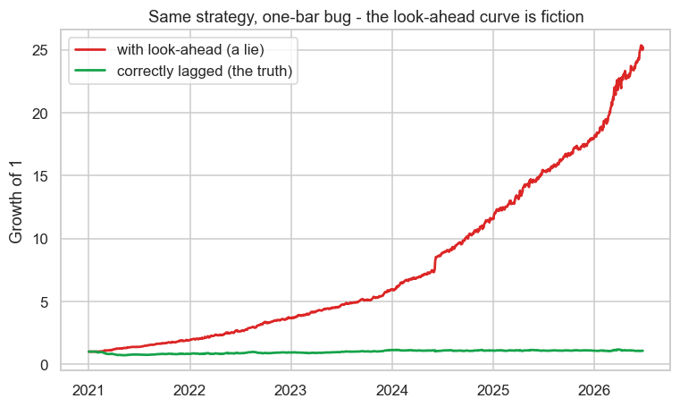
The look-ahead curve rockets to 25x while the honest one crawls to 1.07x - same code, one missing .shift(1). This is why experienced quants are paranoid about timing: every signal must be computable strictly from information available before the bar it trades.

Look-ahead is only the most famous of a whole family of biases that live in the data: survivorship (testing only on the stocks that survived to today), corporate-action distortions (a one-for-one bonus read as a fifty-percent crash), and other point-in-time failures. Each one quietly hands your backtest knowledge the live market would never have given it. Chapter 68 takes them one by one. For now, hold on to the tell: a Sharpe that looks too good to be true almost always is.

In-sample versus out-of-sample

Even with clean data and honest costs, a deeper trap remains: you tuned the strategy on the very data you are now judging it on. Slide a lookback, nudge a threshold, pick the version with the best Sharpe, and the optimizer has quietly fitted the noise in that particular slice of history. The result is in-sample performance, and it is almost always too good, because it includes the strategy's luck as if it were skill.

The discipline that defends against this is the oldest one in the book: hold data back. Fit and tune on an in-sample period, then judge - once - on an out-of-sample period the strategy has never seen (the in-sample versus out-of-sample split first met in the alpha-research process of Chapter 59). If the edge survives untouched data, it might be real. If it falls off a cliff, you were trading noise.

Doing this properly on time series is harder than it sounds, because markets have memory and a careless shuffle leaks the future into the past. The rigorous machinery - walk-forward testing, purged and embargoed cross-validation, and the deflated Sharpe that discounts your search - is the whole of Chapter 69. This chapter just plants the rule: never grade a strategy on data it was allowed to learn from.

Overfitting and data snooping

Out-of-sample discipline can still be defeated by sheer persistence, and that defeat has a name: data snooping. Try enough parameters, indicators, universes and lookbacks, keep the best, and you have manufactured a fluke - even on out-of-sample data, if you peek at it often enough. The uncomfortable truth is that every published backtest you have ever seen is the survivor of a search you were not shown. The more strategies you test, the higher the best one climbs by luck alone - the multiple-testing problem of Chapter 13. A Sharpe of 2 found after a thousand trials is far less impressive than a Sharpe of 1 found on your first honest attempt.

A backtest you can trust

So what does a trustworthy backtest look like? Run this checklist before believing any result, yours or anyone else's:

• Is every signal lagged so it uses only past information? (no look-ahead)
• Is the universe point-in-time, including names that later died or were delisted? (no survivorship - Chapter 68)
• Are realistic costs subtracted on every trade - taxes, spread and impact - so the result is genuinely net?
• Does the edge survive out-of-sample, ideally walk-forward across many periods? (Chapter 69)
• Is the Sharpe deflated for how many variations you tried before keeping this one?
• Is the equity curve lumpy, and is the trade count large enough to be statistically meaningful rather than a handful of lucky bets?
• Is there an economic story for why the edge exists and who is on the losing side of it?

A result that survives all of that has a fighting chance of being real. Everything else is a beautiful lie. The point of a backtest is not to confirm your strategy - it is to disprove it as hard as you can, and respect whatever refuses to die.

With the anatomy and the discipline in place, the next two chapters go deep on the two hardest failure modes. Chapter 68 hunts the biases baked into the data before you write a line of strategy code - look-ahead, survivorship and corporate actions. Chapter 69 then builds validation that respects the clock, so leakage cannot sneak back in through the testing door. Master all three and you will finally have a backtest that describes a market you could actually have traded.